Table of Contents
Relevant: Dividend Discount Models Articles
Gordon Growth Model (GGM)
Gordon Growth Model (GGM), or constant perpetual growth model, is a basic form of the Dividend Discount Model (DDM). Developed in the 1960's by Myron J. Gordon, the model calculates present value by discounting future dividends projected to grow at a constant rate indefinitely.
Formula
where:
- P0 = stock's fair value (at year 0)
- DPS0 = annual dividends per share (at year 0)
- g = perpetual dividend growth rate
- re = discount rate (required rate of return)
Assumptions
- Stable business model: GGM assumes a company with consistent operations, no major strategic shifts, and a predictable market environment.
- Dividend policy and FCFE: Assumes that all free cash flow to equity (FCFE) is distributed as dividends, especially relevant for equity-financed firms, linking dividends to company's free cash flow.
- Constant growth rate: The model expects a stable growth rate for dividends and FCFE, based on historical trends.
- Stable financial leverage: GGM expects unchanged capital structure, ensuring consistent cost of equity and risk profile.
- Perpetual existence: Assumes the company will continue indefinitely, maintaining its competitive position and profitability.
Relevant Applications
- Firms with stable growth rates: Suitable for firms with stable growth rates, typically at or below the economy's nominal rate.
- Firms with high dividend payouts reflecting FCFE: Ideal for companies where a significant portion of FCFE is distributed as dividends.
- Firms with stable leverage: Applicable to companies with consistent leverage ratios.
Limitations
- Constant growth assumption: The steady dividend growth rate assumption may not align with variable growth rates in many companies.
- Input sensitivity: The model is highly sensitive to growth rate and discount rate, where small changes can significantly alter valuation.
- Limited applicability for certain firms: Less suited for companies with irregular dividends, non-dividend payers, or those preferring reinvestment over dividend distribution.
GGM: Formula Inputs
Select between CAPM or your own required rate of return. The CAPM serves as the default cost of equity for all DDMs.
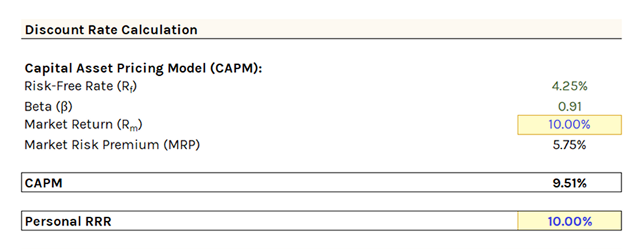
Formula inputs:
- Select the Analysis Year. Outputs the annual DPS and EPS, and updates ROE and DPR.
- Select the dividend calculation method: actual DPS, or EPS × DPR.
- Input the stable growth rate at which DPS and EPS will grow indefinitely. Refer to the DGA tab for guidance.
- This rate must remain below both the discount rate and the nominal growth rate of the economy (usually proxied by the risk-free rate).
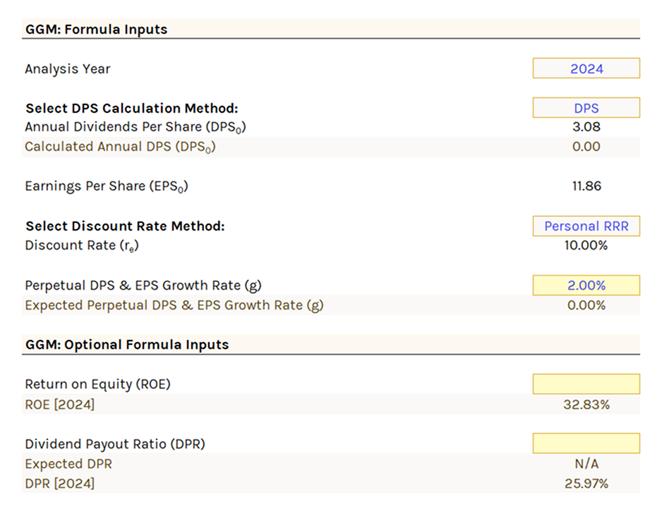
GGM: Formula Outputs
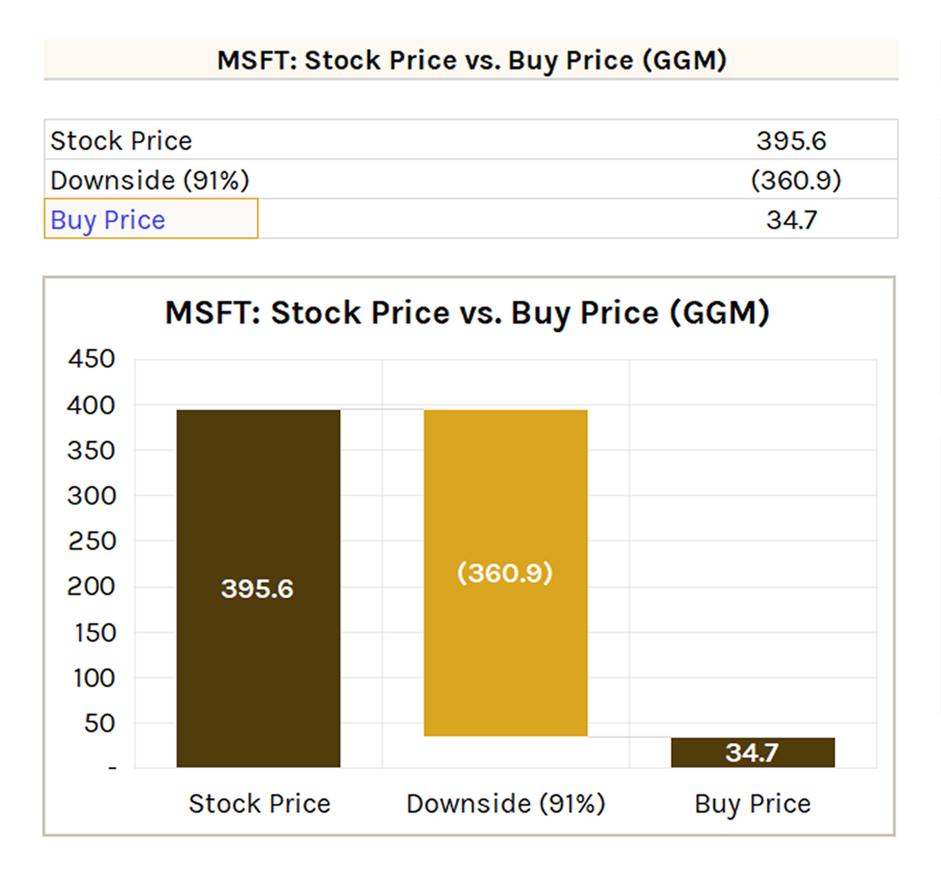
Like the DCF, the GGM outputs the intrinsic value, compares it to the current stock price ($ and % difference), applies a user-defined margin of safety, and outputs a buy price with overvalued/undervalued label.
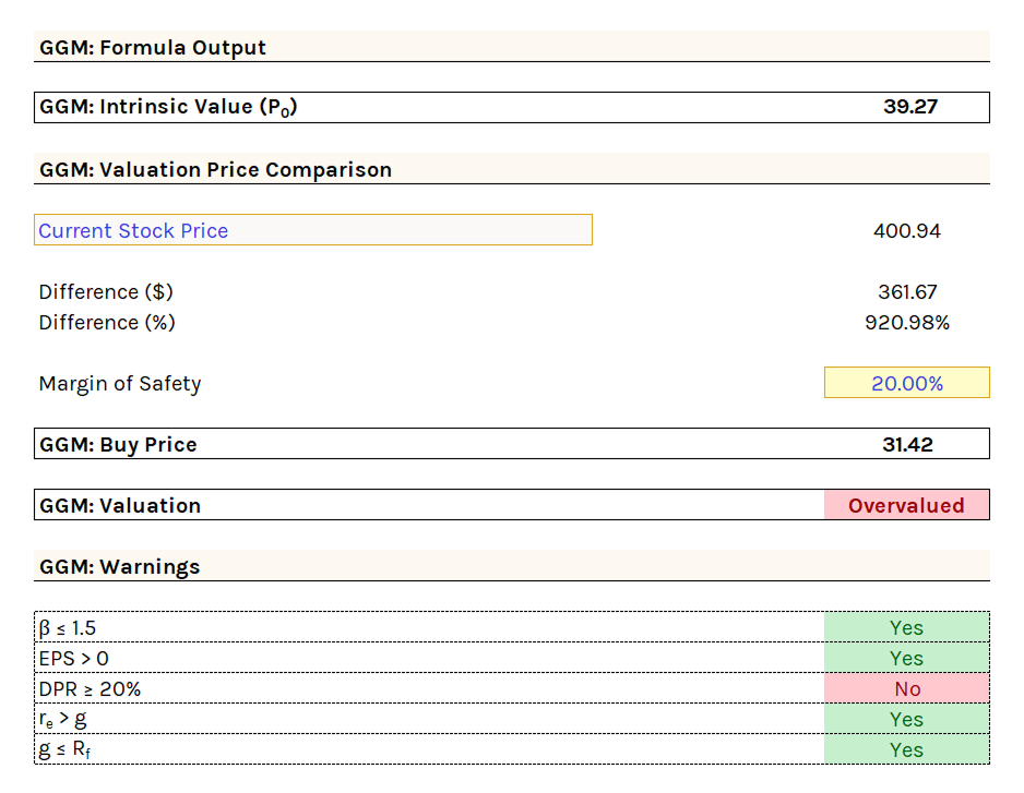
GGM: Warnings
The first three warnings are standard across all DDMs:
- β ≤ 1.5 (volatility check)
- EPS > 0 (dividend sustainability)
- DPR ≥ 20% (sufficient payout)
Two additional warnings evaluate growth rate inputs:
- re > g (discount rate must exceed growth rate)
- g ≤ rf (growth rate should not exceed the risk-free rate)
GGM: Output Chart
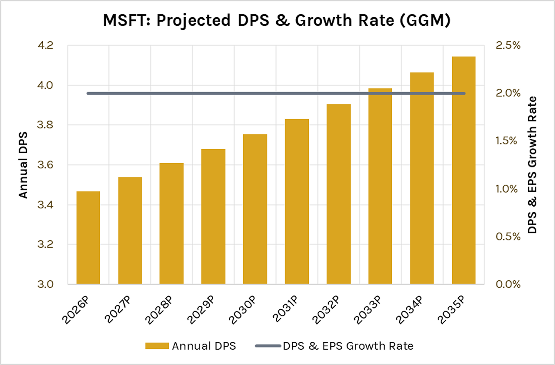
Table shows projected DPS, EPS, growth rate, DPR, and discount rate over the next 10 years.
Chart visualizes annual DPS and DPS & EPS growth rate over the same period.
GGM: Sensitivity Table
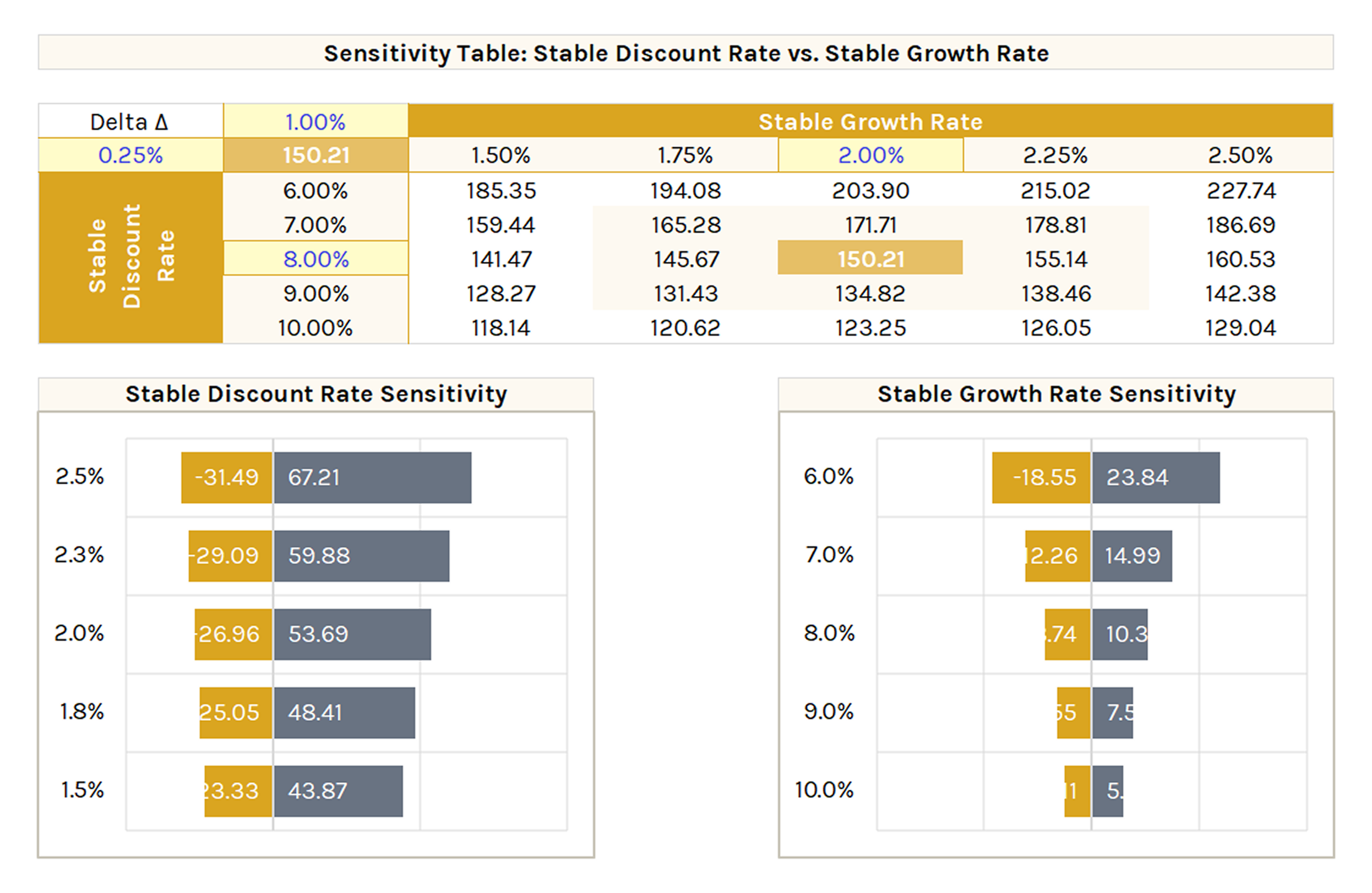
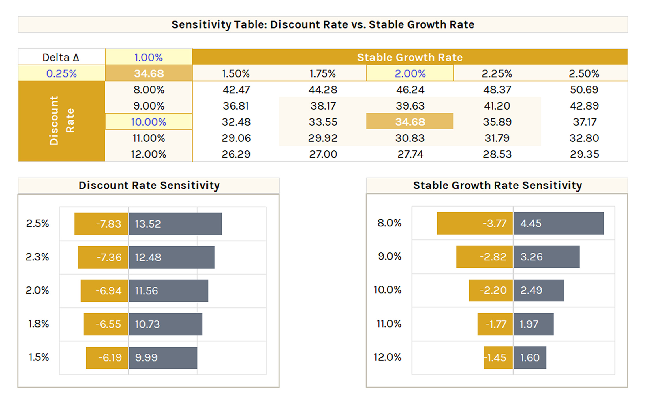
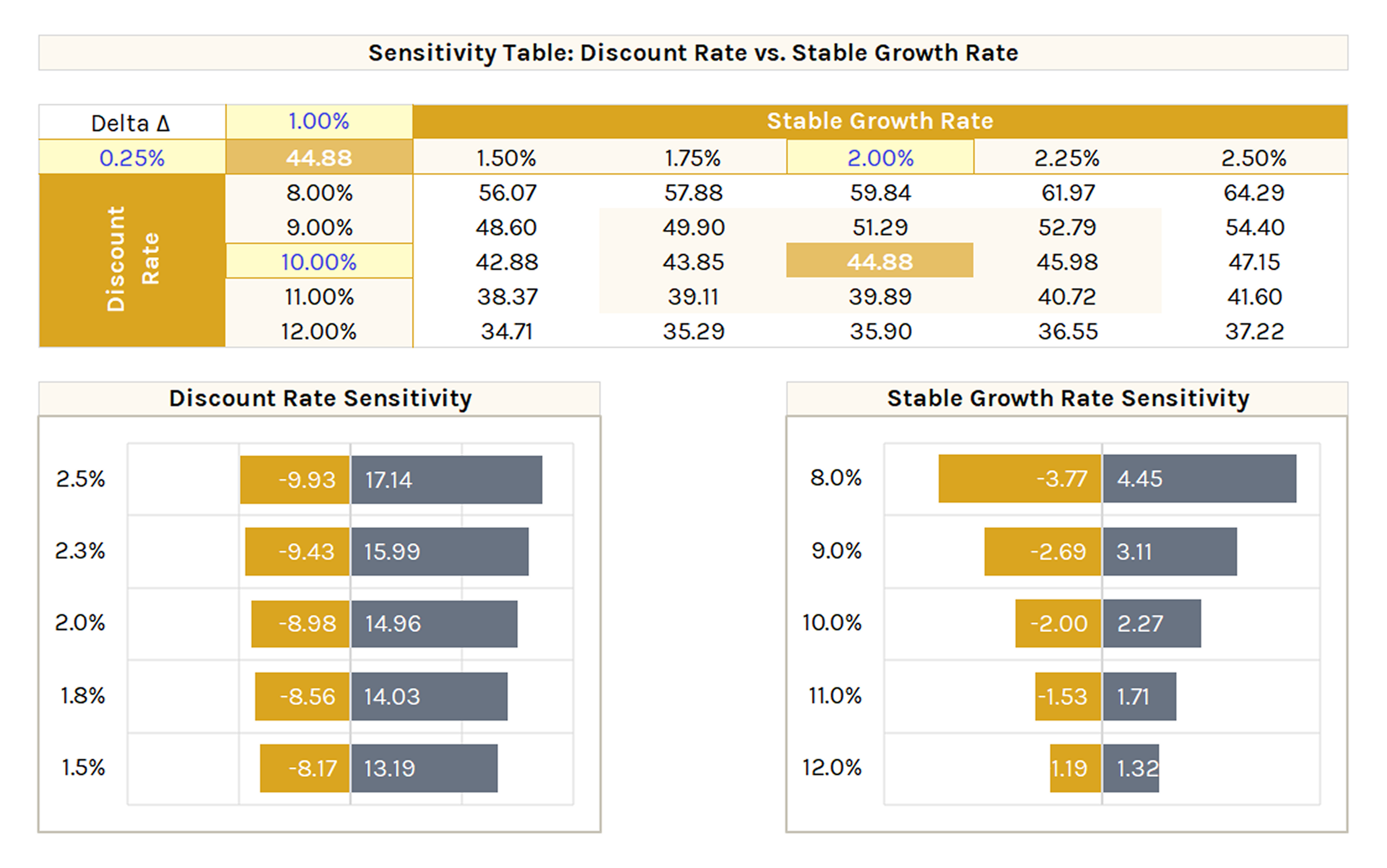
Discount rate vs. stable growth rate. Shows buy prices across different combinations. Enter delta (Δ) increments for each variable.
Waterfall charts below isolate the dollar impact of changing each variable independently from the base case.
Left bar = decrease in buy price, right bar = increase. Useful for seeing which input has more impact on valuation and by how much.
Two-Stage DDM
Two-Stage Dividend Discount Model (DDM) incorporates two distinct phases of dividend growth: initially, a phase of irregular or extraordinary growth, followed by a phase of stable growth into perpetuity.
Present value is calculated by discounting the dividends for each year during the extraordinary growth phase, and then adding the discounted value of dividends expected in the stable growth phase.
Formula
where:
- P0 = stock's fair value (at year 0)
- DPS0 = annual dividends per share (at year 0)
- n = final year of first-stage dividend growth (i.e., when dividend growth changes from g1 to g2)
- g1 = extraordinary high/low dividend growth rate (first stage)
- g2 = perpetual dividend growth rate (second stage)
- re,1 = first growth period discount rate (aka required rate of return)
- re,2 = stable growth period discount rate (aka required rate of return)
Assumptions
- Extraordinary growth phase: Characterized by high, low, or negative growth rates, reflecting unique company challenges and strategies like expansion or restructuring.
- Transition to stable growth: Post extraordinary growth, the company shifts to sustainable growth, aligning with industry and economic averages.
- Variable dividend payout ratio: Changes with growth phase; lower in high growth due to reinvestment, higher in stable growth.
- Adjustment of firm characteristics in stable phase: Characteristics like beta and return on equity adjust to reflect stability; beta normalizes, and return on equity aligns with stable company levels.
Relevant Applications
- Effective for diverse growth phases: Suitable for companies with varied growth patterns, including high-growth firms transitioning to normal rates and those with moderate initial growth.
- Mature companies with consistent dividends: Aligns well with mature companies having a history of consistent dividends and moderate growth, capturing their shift to a stable phase.
- High dividend payout ratios and residual cash flow distribution: Applicable to firms with high dividend payout ratios distributing substantial residual cash flows as dividends, indicating a move from reinvestment to shareholder distributions.
Limitations
- Defining the length of extraordinary growth phase: Accurately determining the duration of the extraordinary growth phase is complex, introducing uncertainty in valuation due to the model's sensitivity to this period.
- Abrupt transition to stable growth: Assumes an immediate shift from extraordinary to stable growth, which oversimplifies real-world gradual transitions, potentially leading to inaccuracies.
- Predicting future dividend growth: Forecasting dividend growth in the initial high growth stage is challenging, as firms often reinvest earnings rather than pay substantial dividends.
Two-Stage DDM: Formula Inputs
Two discount rate stages are available (one per growth phase).
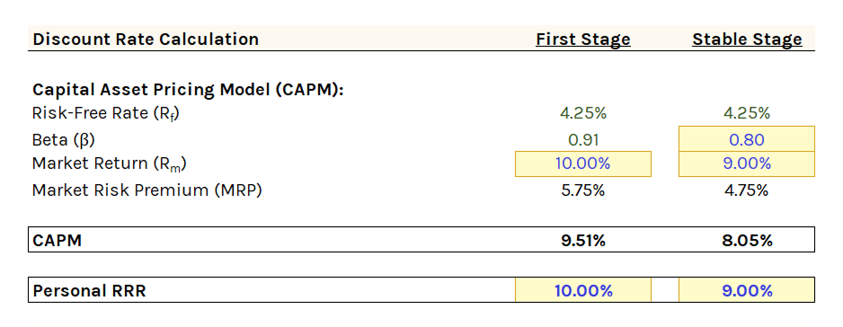
Formula inputs are similar to GGM with key differences:
- DPS calculation method (DPS or EPS × DPR) is in the formula outputs section.
- Select the number of years for the initial extraordinary growth phase (1 to 10 years).
- Two stages require separate selections for: discount rate method, ROE, DPS & EPS growth rate, and DPR.
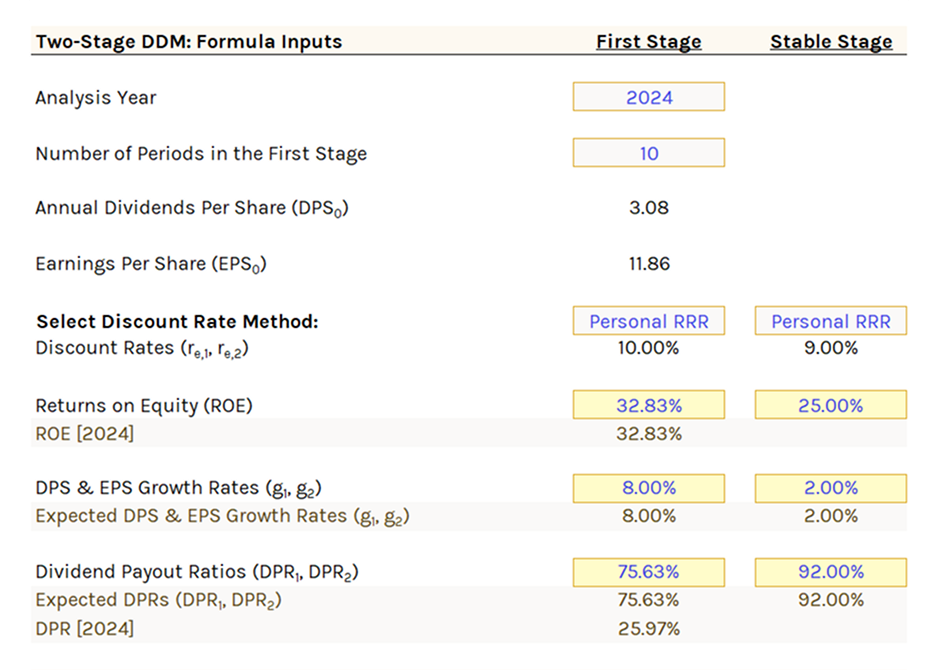
In a standard Two-Stage DDM, the stable stage (vs. the first stage) has a lower discount rate, lower ROE, lower growth rate, and higher DPR. For companies transitioning from low/negative growth to stable growth, these inputs reverse.
Two-Stage DDM: Formula Outputs
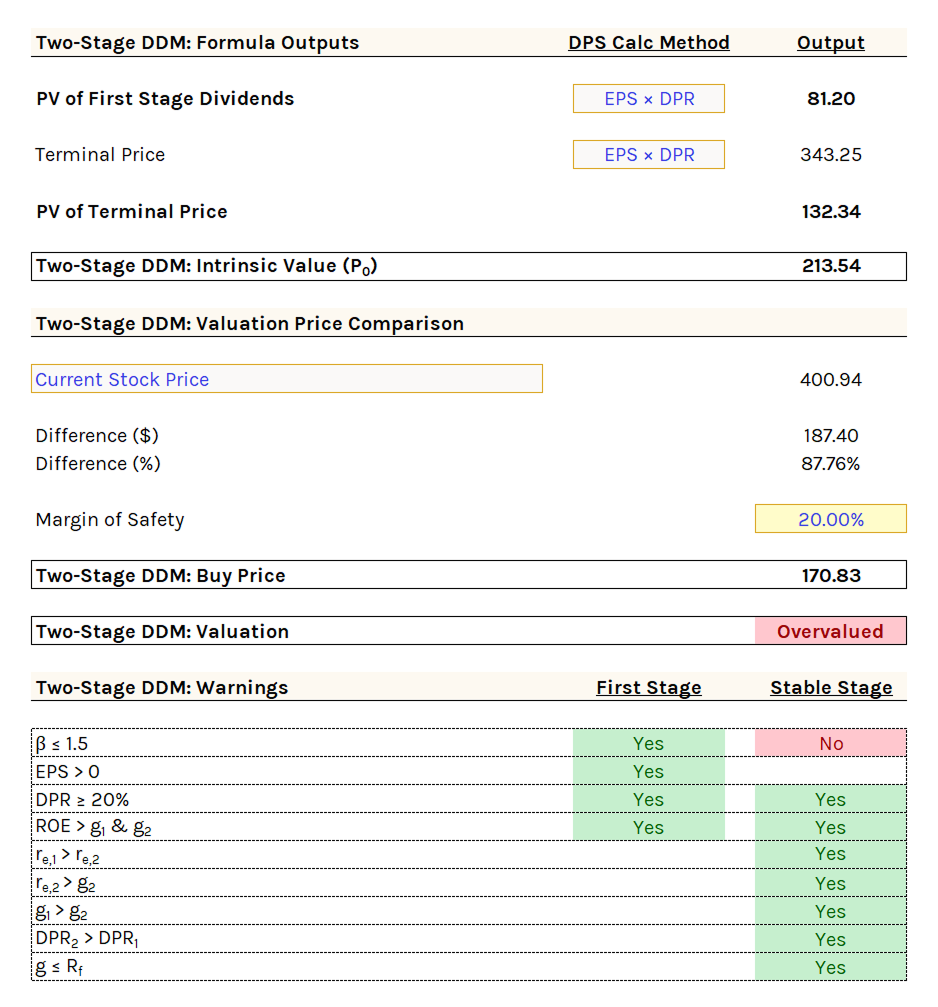
Shows the PV calculation of both the first stage and stable stage dividends.
DPS calculation method toggles:
- DPS: Directly input expected DPS & EPS growth, disregarding EPS, DPR, and ROE.
- EPS × DPR (recommended): Calculates dividends based on earnings and payout ratio, assuming dividends and earnings grow in tandem.
Same margin of safety and buy price output as GGM.
Two-Stage DDM: Warnings
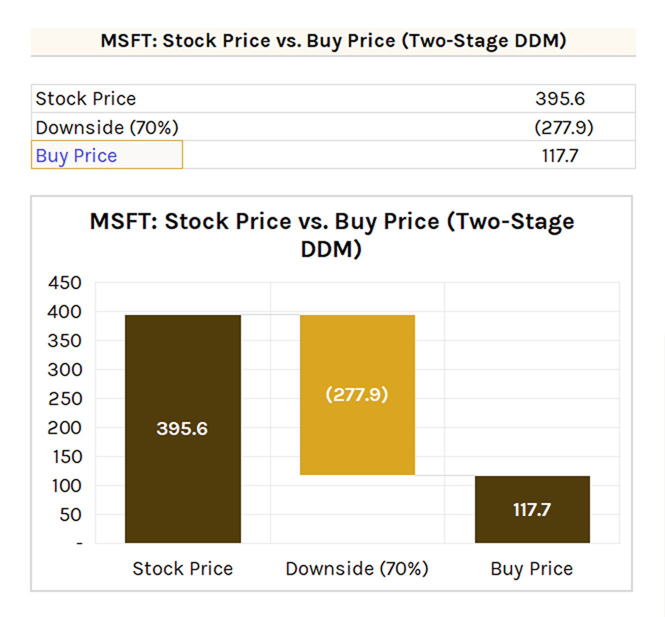
Same standard warnings as GGM, plus:
- ROE > g1 & g2 (ROE must support projected growth rates)
- re,1 > re,2 (first stage discount rate should exceed stable stage)
- g1 > g2 (first stage growth should exceed stable growth)
- DPR2 > DPR1 (stable stage payout should exceed first stage)
Two-Stage DDM: Output Chart
Two tables:
- First Stage: Projects DPS, EPS, growth rate, DPR, and discount rate over the initial stage (up to 10 years). PV of first stage dividends is calculated.
- Stable Stage: Mirrors the GGM table for the subsequent 10 years.
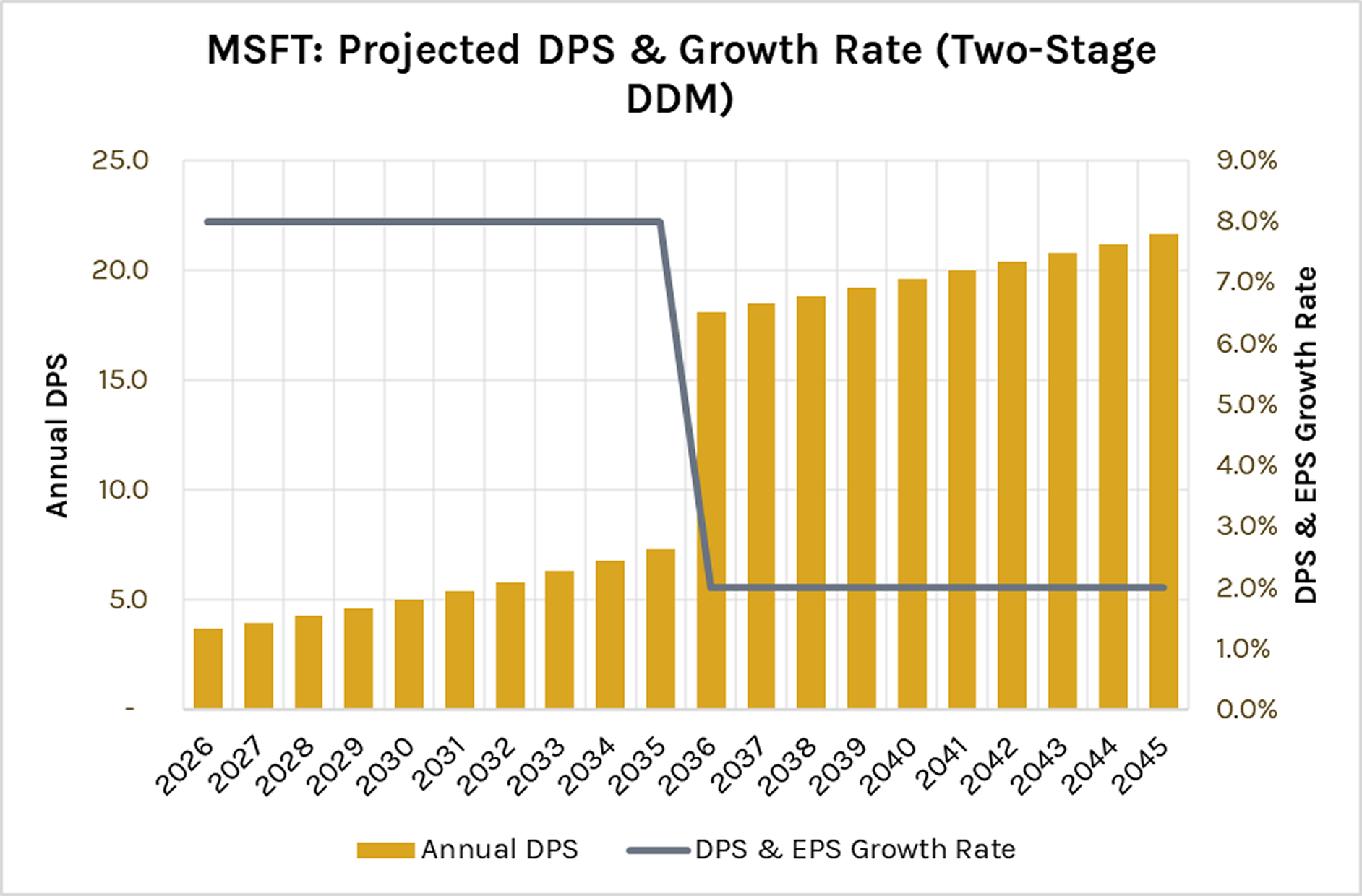
Chart visualizes annual DPS and DPS & EPS growth rates over up to 20 years.
Two-Stage DDM: Sensitivity Table
Stable discount rate vs. stable growth rate. Same structure as GGM.
The discount rate refers to the stable phase discount rate, not the first stage.
H-Model
H-Model, an adaptation of the Two-Stage DDM, was introduced by Fuller and Hsia in 1984. It features a gradual transition from extraordinary to stable growth, contrasting the immediate shift seen in the traditional model. This is followed by a phase of stable growth into perpetuity.
Present value is calculated by discounting dividends during the extraordinary growth phase, and then adding the discounted dividends from the stable growth phase.
Formula
where:
- P0 = stock's fair value (at year 0)
- DPS0 = annual dividends per share (at year 0)
- H = half life of anticipated transition period
- g1 = increasing/declining dividend growth rate (first stage)
- g2 = perpetual dividend growth rate (second stage)
- re = discount rate (aka required rate of return)
Assumptions
- Extraordinary growth phase: Assumes company's earnings and dividends are experiencing an extraordinary growth phase.
- Linear change in earnings: Earnings growth is expected to change linearly over a period indicated as 2H.
- Stable dividend payout and cost of equity: Dividend payout ratio and cost of equity remain constant throughout the transition phase, despite changing growth rates.
- Steady state growth post-transition: Anticipates stable dividend growth indefinitely after the initial declining phase.
Relevant Applications
- Effective for diverse growth phases: Appropriate for businesses with different growth trends, this method is applicable to high-growth companies moving to regular growth rates and those experiencing low/negative initial growth.
- Companies in transition: Ideal for larger firms transitioning from an extraordinary growth phase to a stable rate, such as those facing diminishing competitive advantages.
- Firms with temporary growth spurts: Suited for companies with temporary growth surges, such as those with new products or first-mover advantages.
Limitations
- Rigidity in growth rate change: Assumes a uniform linear change in growth rates (2H), which may not reflect actual dividend patterns with deviations from linear change.
- Constant payout ratio and cost of equity assumption: Presumes constant dividend payout ratio and cost of equity during both phases, not accounting for changes companies might make as growth rates decrease.
- Impact of long extraordinary growth periods: Less effective for prolonged extraordinary growth phases, leading to disparities between initial extraordinary growth and long-term sustainable rates.
H-Model: Formula Inputs
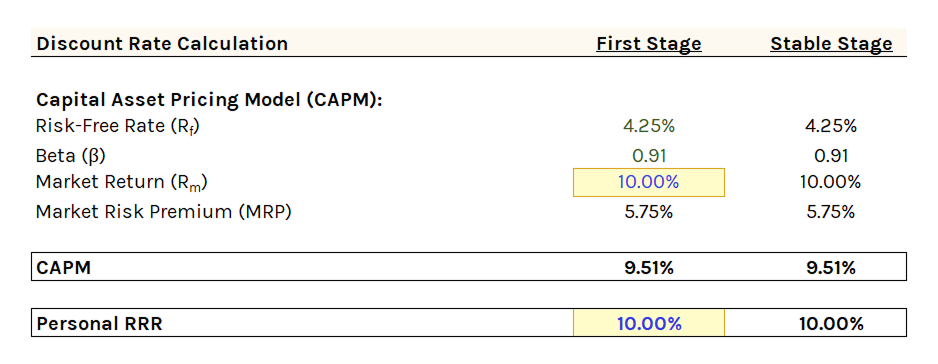
Discount rate remains constant across both stages (unlike the Two-Stage DDM).
Formula inputs are similar to the Two-Stage DDM with key differences:
- ROE and DPR are optional inputs (like the GGM).
- Discount rate, ROE, and DPR remain constant across both stages.
- Only the DPS & EPS growth rates change between stages.
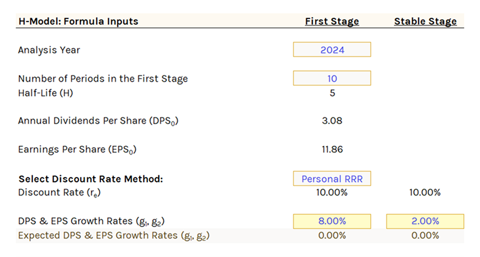
- Selection of first stage periods determines the half-life output.
H-Model: Formula Outputs
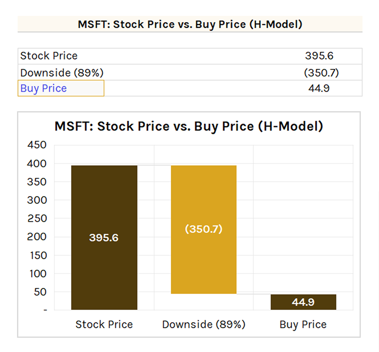
Shows the PV calculation of both the initial and stable stage dividends.
Default DPS calculation method should be "DPS" (not "EPS × DPR"), aligning with the H-Model's assumption of constant discount rates, ROEs, and DPRs across stages.
Same margin of safety and buy price output as previous DDMs.
H-Model: Warnings
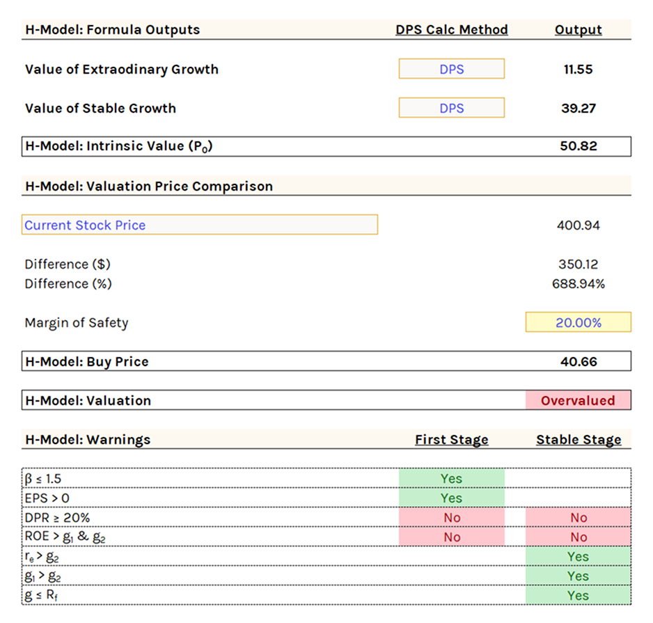
Same as Two-Stage DDM, excluding warnings about changing discount rates, ROEs, and DPRs (which are constant in the H-Model).
H-Model: Output Chart
Two tables similar to Two-Stage DDM.
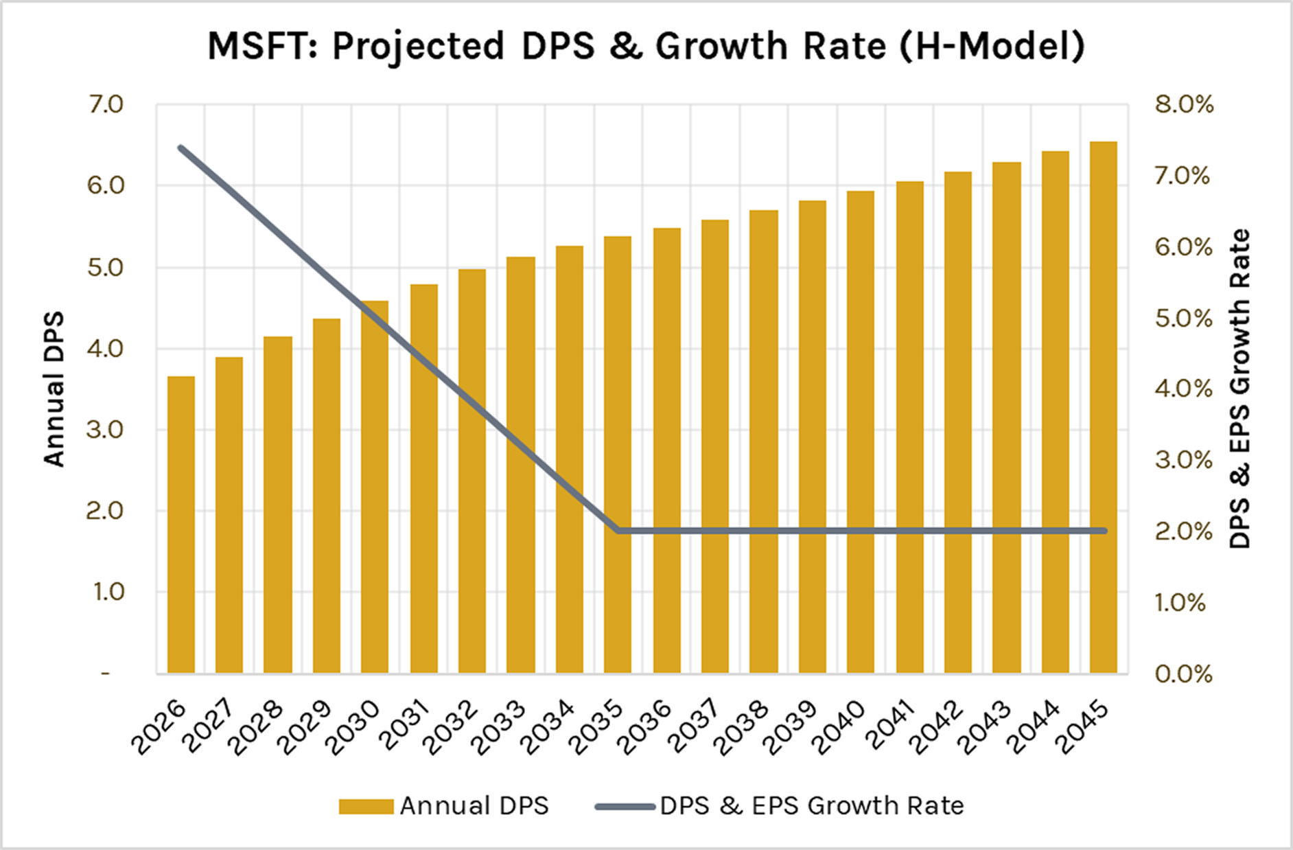
Key difference: DPS & EPS growth rate changes linearly over the first stage rather than remaining constant. Stable stage mirrors the GGM table.
Chart visualizes annual DPS and the gradual change in DPS & EPS growth rates over up to 20 years.
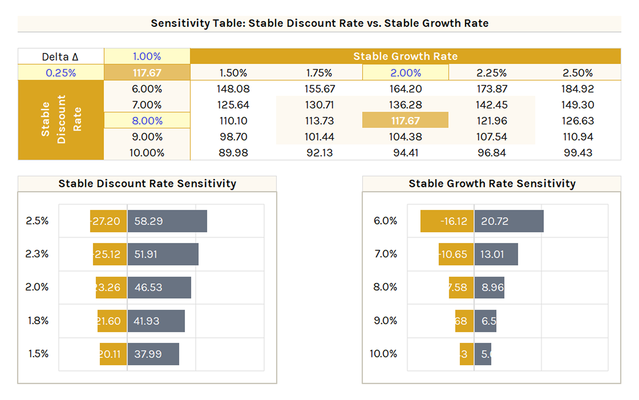
H-Model: Sensitivity Table
Discount rate vs. stable growth rate. Same structure as GGM.
Three-Stage DDM
Three-Stage Dividend Discount Model (DDM) combines elements from the Two-Stage DDM and the H-Model, making it the most intricate DDM. This model encompasses three distinct growth phases: initial extraordinary growth, a transitional change in growth, and a final phase of stable growth into perpetuity.
Present value is calculated by discounting dividends across all phases: initial extraordinary growth, a transitional phase with changing rates, and the final stable growth phase.
Formula
where:
- P0 = stock's fair value (at year 0)
- DPSt = annual dividends per share (in year t)
- EPSt = earnings per share (in year t)
- DPR1 = dividend payout ratio in extraordinary growth phase
- DPR2 = dividend payout ratio in stable growth phase
- n1 = final year of the extraordinary growth phase where the dividend growth rate is g1
- n2 = year when the stable growth rate g2 takes effect after the transition phase
- g1 = extraordinary high/low dividend growth rate (first stage)
- g2 = perpetual dividend growth rate (third/final stage)
- re,1 = discount rate (aka required rate of return) in extraordinary growth phase
- re,2 = discount rate (aka required rate of return) in transition phase
- re,3 = discount rate (aka required rate of return) in stable growth phase
Assumptions
- Initial extraordinary growth phase with defined duration: Begins with high, low, or negative growth due to factors like expansion or restructuring, where defining the duration is crucial for valuation.
- Linear transition to stable growth: Assumes a gradual shift in growth and discount rates, with changing dividend payout ratios, reflecting adjusted risk and reinvestment needs as the company matures.
- Correlation between dividend payout ratio and growth rate: Suggests variable dividend payout ratios depending on growth phases, with higher ratios in stability and lower during high growth.
- Risk profile, cost of capital, and financial policy adjustments: Expects adjustments in risk profile, cost of capital, and financial policies across growth stages, with a decreasing cost of equity moving towards stability.
Relevant Applications
- Dividend alignment and initial extraordinary growth: Suitable for companies in extraordinary growth phases with dividends closely aligned with free cash flow to equity (FCFE).
- Gradual growth rate decline and stable leverage: Excels in capturing gradual growth rate reductions in maturing firms, coupled with stable leverage, reflecting consistent financial strategies.
- Adaptability to payout and risk profile shifts: Ideal for fast-growing firms undergoing changes in dividend policies and risk profiles, capturing their transition to sustainable growth.
- Realistic business lifecycle representation: Effectively mirrors business cycles, especially for companies initially experiencing high growth due to innovation or market dominance, adapting to their evolving growth dynamics.
Limitations
- Complexity and sensitivity in estimating inputs: Requires precise estimations of inputs like payout ratios, growth rates, and betas, with sensitivity to these estimates leading to valuation inaccuracies.
- Challenges in defining growth phase durations: Determining the length of growth phases, particularly the extraordinary growth and transition periods, is challenging and prone to misvaluation due to the difficulty in translating qualitative analyses into exact timeframes.
- Oversimplification of growth transition: The assumption of a linear transition from high to stable growth may not reflect the complex and sometimes non-linear nature of real-world growth changes.
- Predicting future dividend growth: Forecasting dividend growth during the early high growth phase can be difficult, since companies typically reinvest profits instead of distributing significant dividends.
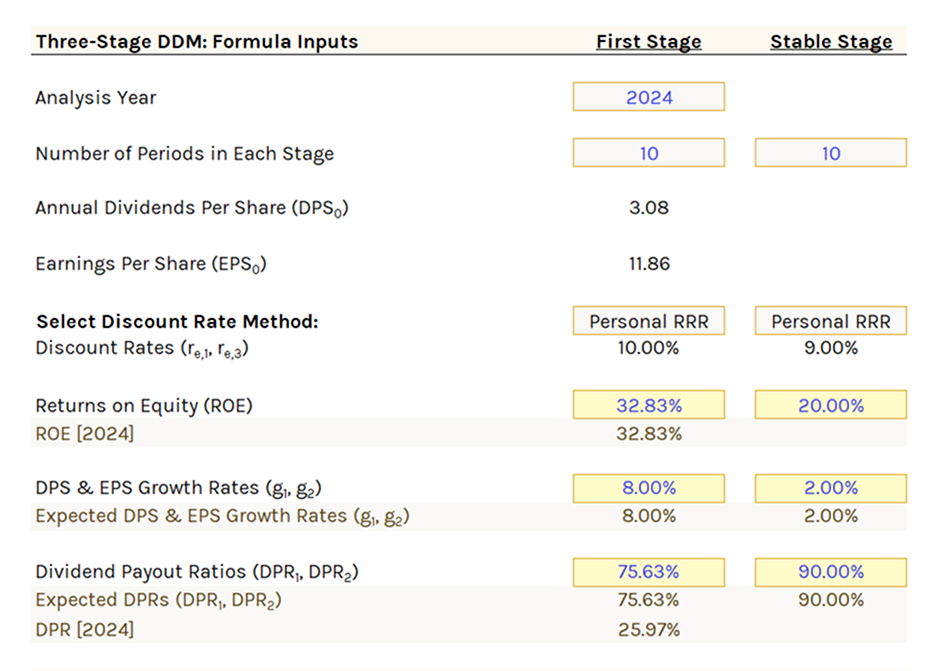
Three-Stage DDM: Formula Inputs
Discount rate calculation is identical to the Two-Stage DDM.
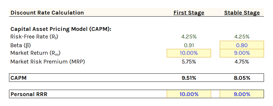
Formula inputs are identical to the Two-Stage DDM, with an additional dropdown to select the number of periods in the transition stage.
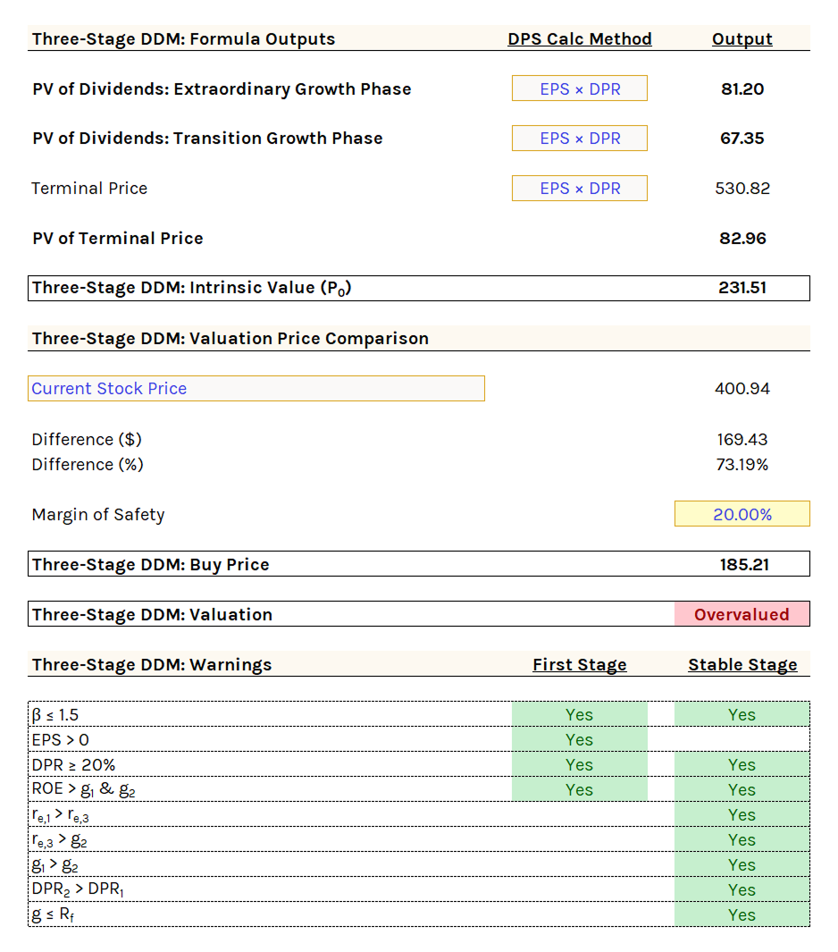
Three-Stage DDM: Formula Outputs
Shows the PV calculation of the first stage, transition stage, and stable stage dividends.
"EPS × DPR" is the recommended DPS calculation method (like the Two-Stage DDM).
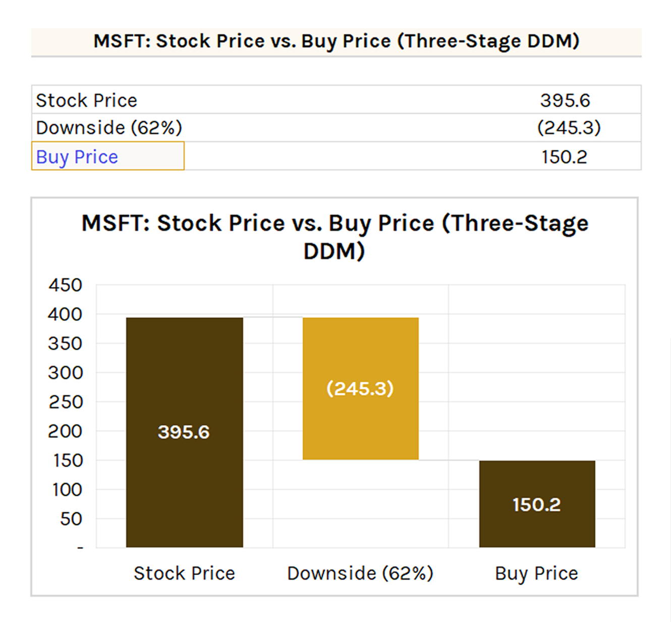
Same margin of safety and buy price output as previous DDMs.
Three-Stage DDM: Warnings
Identical to the Two-Stage DDM, using "re,3" instead of "re,2."
Three-Stage DDM: Output Charts
Three tables:
- First Stage: Same as Two-Stage DDM.
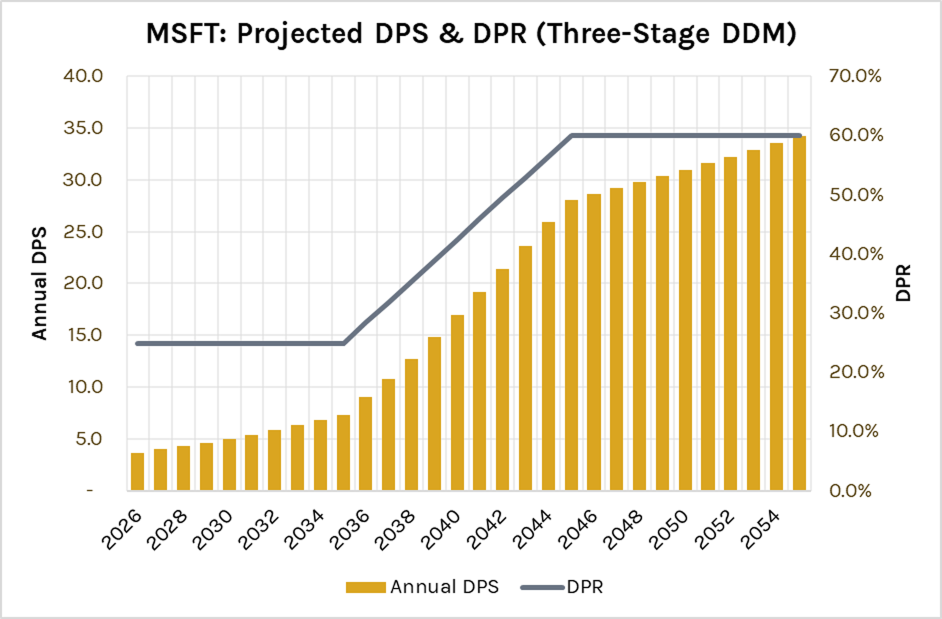
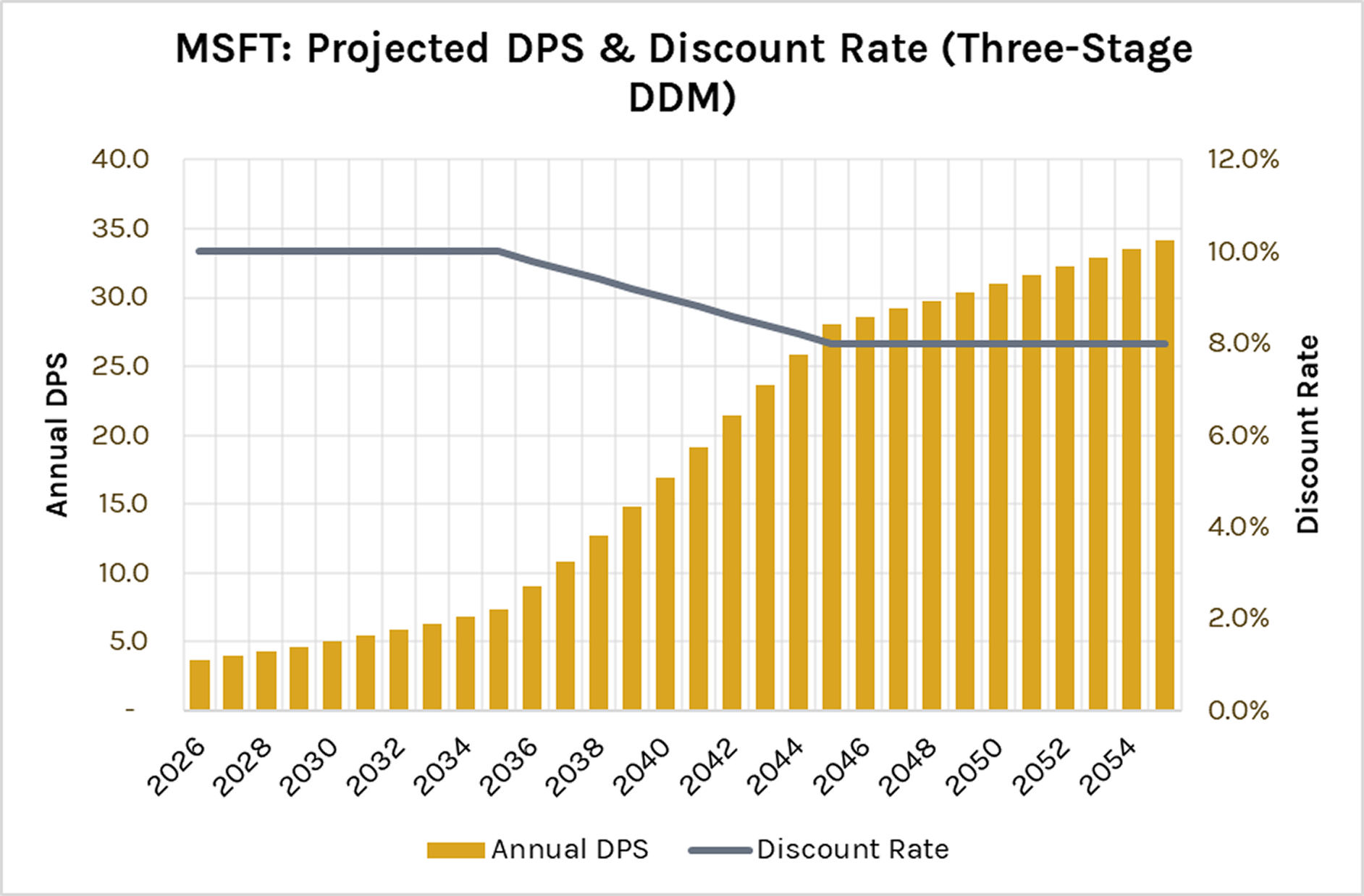
- Transition Stage: Features linearly changing DPS & EPS growth rates, DPRs, and discount rates with cumulative PV calculations.
- Stable Stage: Mirrors the GGM table for the subsequent 10 years.
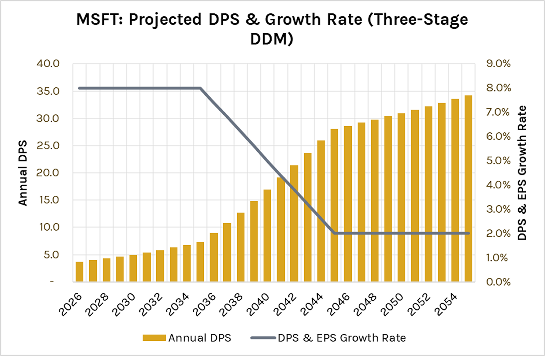
Three charts visualize annual DPS alongside DPS & EPS growth rates, DPRs, and discount rates over up to 30 years.
Three-Stage DDM: Sensitivity Table
Stable discount rate vs. stable growth rate. Same structure as GGM.
The discount rate refers to the stable phase discount rate.