

Table of Contents
Relevant: Discounted Cash Flow Articles
DCF Overview
Discounted Cash Flow (DCF) is a valuation method that estimates a company's intrinsic value by calculating the present value of projected future cash flows, accounting for both the time value of money and the risk of generating these cash flows.
Formula
where:
- P0 = stock's fair value (at year 0)
- n = number of periods (years) for which cash flows are projected
- CFt = cash flow (at time t)
- re = discount rate (aka required rate of return)
- TV = terminal value (at the end of period n)
Assumptions
- Cash flow projections: Relies on accurate cash flow projections based on future performance assumptions.
- Constant discount rate: Assumes a relatively stable and suitable discount rate over the projection period.
- Terminal value: Incorporates a terminal value representing cash flows beyond the explicit projection period.
- Stable financial leverage: Expects unchanged capital structure, ensuring consistent risk profile and discount rate throughout the projection period.
Relevant Applications
- Non-dividend-paying companies: Ideal for valuing companies that don't pay dividends, focusing on free cash flows.
- Companies with low dividend payout ratios: Also suitable for companies with low dividend payout ratios by considering total free cash flows.
- Alignment of free cash flow and profitability: Suitable for companies with projected free cash flows aligning closely with profitability within the forecast period.
- Majority ownership or control: Relevant for investors with controlling interest, assessing value based on discretion over equity cash flows.
Limitations
- Input sensitivity: Valuations are highly sensitive to assumptions about growth rates, discount rates, and terminal values.
- Reliance on projections: Accuracy depends on the reliability of cash flow projections.
- Difficulty in estimating terminal value: Requires assumptions about long-term growth rates and competitive position.
- Limited applicability for certain firms: Less suitable for early-stage companies, firms with negative cash flows, firms with high dividend payout ratios, or volatile industries.
DCF Formula Inputs
Configure the DCF Model:
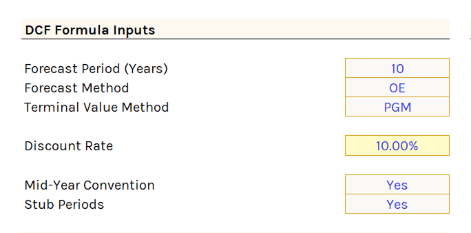
Forecast Period (Years)
Select between 1 to 10 years. Determines how many years of cash flows are forecasted.
The ideal forecast period extends to when the company reaches a steady state or normalized level of financial performance.
Longer forecast periods introduce greater estimation error.
Forecast Method
Three cash flow forecast methods available:
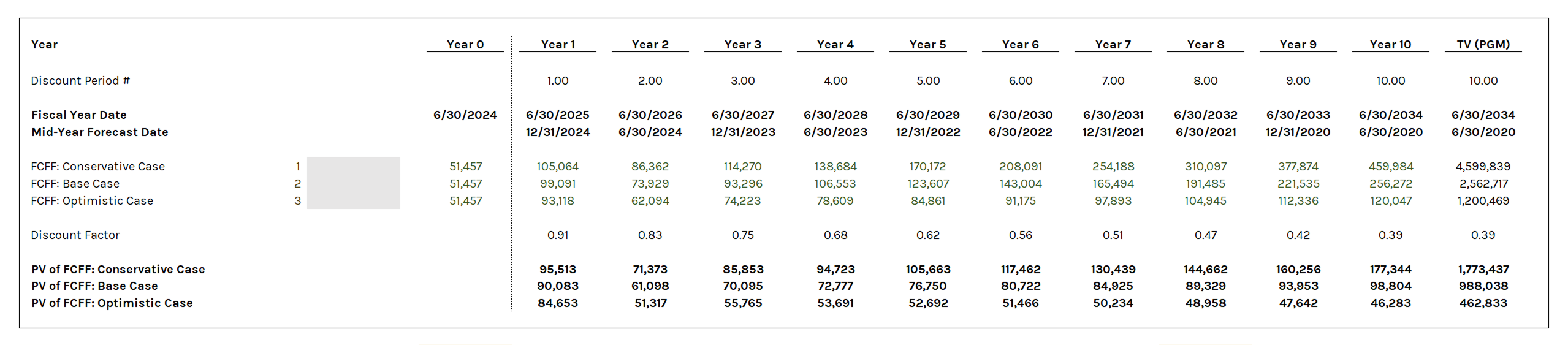
FCFF (Free Cash Flow to the Firm)
Unlevered cash flows available to all investors (debt, preferred, and equity holders) before interest payments. Standard approach in most DCF models because it values the entire company before considering how it's financed.
Selecting "FCFF" pulls forecasted values directly from the FCFF tab, including conservative, base, and optimistic scenarios.
OE (Owners Earnings)
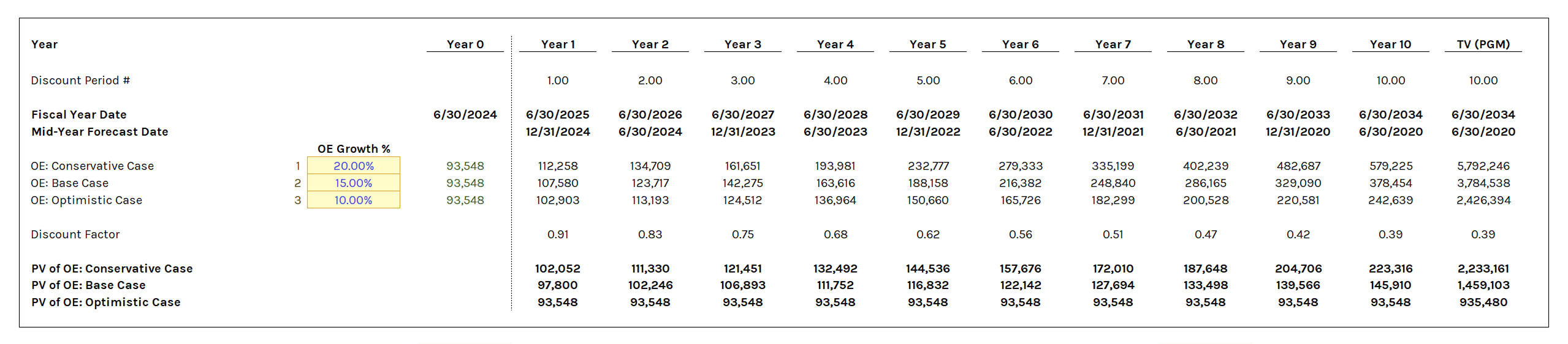
Cash flows available to equity owners after all necessary maintenance CapEx.
Selecting "OE" makes three input cells visible for forecasting growth rates across the conservative, base, and optimistic cases. The year zero OE number comes from the OE tab.
DEPS (Diluted Earnings Per Share)
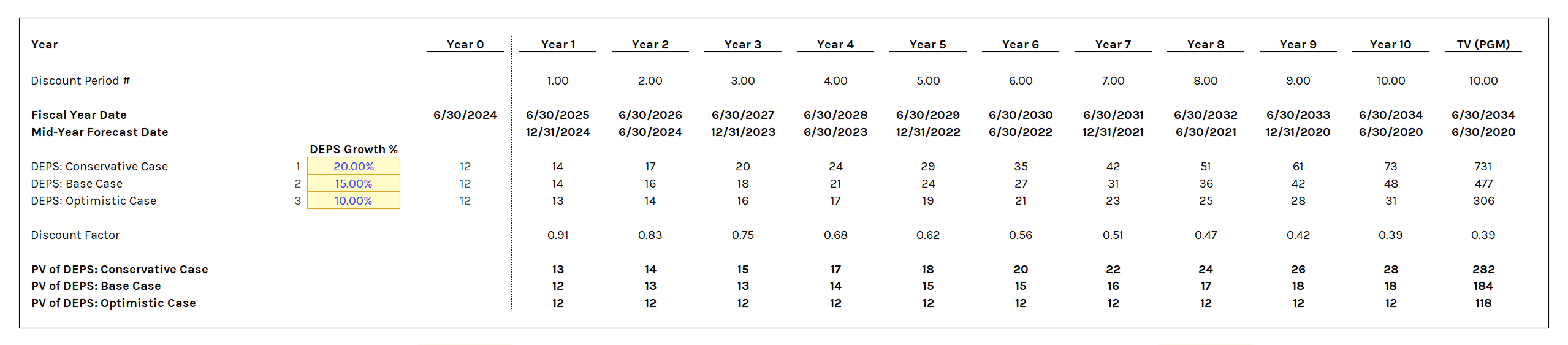
Accounting earnings divided by diluted shares outstanding.
Less accurate than FCFF or OE because it includes non-cash items and doesn't reflect actual CapEx or working capital changes. Useful for quick screening or when free cash flows are negative.
Same functionality as OE, except it uses the last fiscal year's DEPS from the income statement.
Terminal Value Method
Terminal value represents the estimated value of the investment beyond the forecast period. Two methods available:
Perpetual Growth Method (PGM)
Assumes the company grows cash flows at a stable rate indefinitely (at or below GDP growth):
TV = CFn × (1 + g) / (r - g)
where:
- TV = terminal value
- CFn = cash flow in final explicit forecast year
- g = perpetual growth rate
- r = discount rate
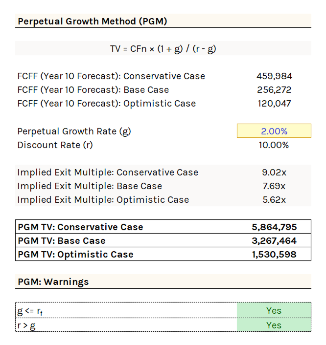
Note: CFn depends on your Forecast Period selection (1-10 years) and Forecast Method (FCFF, OE, or DEPS).
PGM Constraints
- Growth rate constraint: g cannot exceed the nominal growth rate of the economy. The proxy is typically the long-term risk-free rate, since both contain the same inflation component.
- Discount rate relationship: g must be below r. Otherwise the denominator becomes negative, producing a meaningless terminal value.
- Negative growth: g can be negative, implying the firm gradually liquidates itself (appropriate for structurally declining businesses).
Exit Multiple Method (EMM)
Applies a market-based multiple to the terminal year financial metric:
TV = MetricTerm × Exit Multiple
where:
- TV = terminal value
- MetricTerm = terminal year financial metric
- Exit Multiple = market-based valuation multiple from comparable companies (usually based on LTM/NTM multiples)
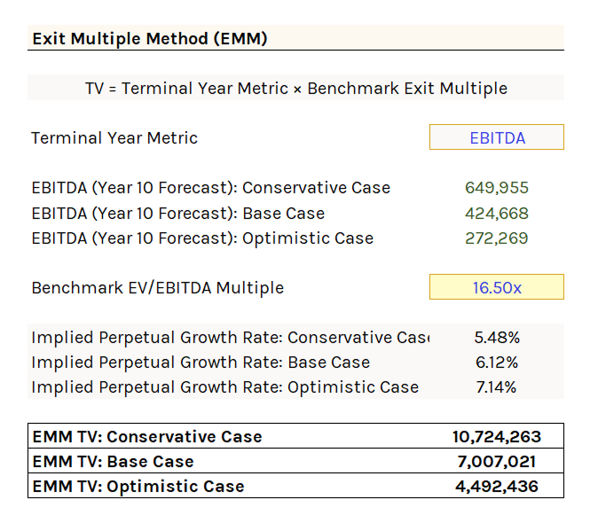
You must input estimate of the benchmark multiple, which can be based on Revenue, EBIT, EBITDA, or FCFF:
The terminal year metric will depend on your Forecast Period selection (1-10 years) and the metric you choose (Revenue, EBIT, EBITDA, or FCFF).
Note: EMM is not compatible with "OE" or "DEPS" forecast methods since terminal year metrics are sourced from the FCFF tab.
Cross-Checking PGM and EMM
The model provides implied growth rates (from EMM) and implied multiples (from PGM) as sanity checks.
Implied Perpetual Growth Rate (From EMM)
Implied Growth Rate = ((TVEMM × r) - CFTerm) / (TVEMM + CFTerm)
where:
- TVEMM = terminal value (exit multiple method)
- r = discount rate
- CFTerm = terminal year cash flow
If the implied growth rate is unreasonably high or low, revisit your exit multiple assumptions.
Implied Exit Multiple Formula (From PGM)
Implied Multiple = TVPGM / MetricTerm
where:
- TVPGM = terminal value (perpetual growth method)
- MetricTerm = terminal year financial metric
If the implied multiple is unreasonably high or low vs. current trading multiples, revisit your perpetual growth rate assumption.
Note: If "Mid-Year Convention" is enabled, these formulas adjust to account for mid-year timing. See the mid-year convention formulas below.
Discount Rate
The rate at which future cash flows are discounted back to present value.
- Forecasting FCFF: Use WACC (=WACC), risk-free rate (=RF_Rate_10YR), or your own required rate of return.
- Forecasting OE or DEPS: Use CAPM (=CAPM), Modified CAPM (=Modified_CAPM), risk-free rate (=RF_Rate_10YR), or your own required rate of return.
FCFF is unlevered (before interest), so it uses WACC which reflects the blended cost of all capital sources. OE and DEPS are levered (after debt obligations), so they use an equity discount rate like CAPM.
Mid-Year Convention and Stub Periods
Four DCF discounting approaches are available:
- FY-End Discounting: Assumes all cash flows occur at the end of each fiscal year (FY-end).
- Mid-Year Convention: Assumes cash flows occur at the midpoint of each fiscal year rather than at FY-end.
- FY-End With Stub Periods: Adjusts for partial periods when the valuation date doesn't align with the FY-end.
- Mid-Year Convention With Stub Periods: Combines both mid-year and stub period adjustments for more precise cash flow timings.
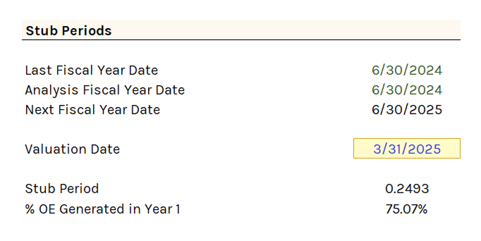
Recommended to enable both mid-year convention and stub periods for most companies. The model adjusts discount periods and terminal value calculations automatically.
FY-End Discounting
Assumes all cash flows occur at fiscal year-end.
- Mid-Year Convention: No
- Stub Periods: No
Discount Factor = 1 / (1 + r)n
where:
- r = discount rate
- n = number of periods into the future
Terminal value uses the same discount factor as the final year's cash flows.
Mid-Year Convention
Assumes cash flows occur at the midpoint of each fiscal year rather than year-end, resulting in a slightly higher valuation.
- Mid-Year Convention: Yes
- Stub Periods: No
Mid-Year Discount Factor = 1 / (1 + r)(n - 0.5)
Impact on terminal value:
- EMM: Discounted at "n" periods (one-time transaction at period end).
- PGM: Discounted at "(n - 0.5)" periods (perpetual cash flows assumed at mid-year).
Mid-Year Cross Check Formulas
Implied Growth Rate (Mid-Year) = [(TVEMM × r) - CFTerm × (1 + r)0.5] / [TVEMM + CFTerm × (1 + r)0.5]
where:
- TVEMM = terminal value (exit multiple method)
r = discount rate
CFTerm = terminal year cash flow
Implied Multiple (Mid-Year) = TVPGM × (1 + r)0.5 / MetricTerm
where:
- TVPGM = terminal value (perpetual growth method)
r = discount rate
MetricTerm = terminal year financial metric
FY-End Stub Periods
Adjusts for partial first-year periods when the valuation date falls within the first forecast year.
- Mid-Year Convention: No
- Stub Periods: Yes
Steps:
- Input the Valuation Date. Must be before the next fiscal year date.
- The model calculates the stub fraction (days between valuation date and next FY-end / days in fiscal year).
- Year 1 cash flow is adjusted: CF1 × Stub Period.
- Discount periods adjust accordingly: first year uses the stub period, subsequent years add 1.0 (s + 1, s + 2, etc.).
Terminal value uses the same discount period as the final year's cash flow.
Mid-Year Convention With Stub Periods
Combines both adjustments. Recommended for most companies.
- Mid-Year Convention: Yes
- Stub Periods: Yes
Mid-year convention with stub periods adjusts discount periods to reflect both the partial first forecast year and that cash flows occur at mid-year.
Discount period adjustments:
- First forecast year: s / 2 (midpoint of stub period).
- Second forecast year: s + 0.5 (midpoint of first full year).
- Subsequent years: add 1.0 to the previous period.
Impact on terminal value:
- EMM: Final year's discount period plus 0.5 years.
- PGM: Same discount period as the final year's cash flow.
DCF Formula Outputs
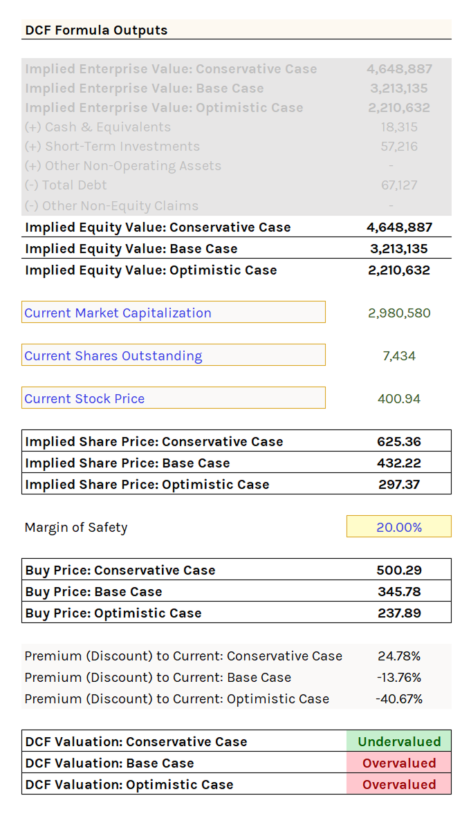
Implied Share Price
The calculation differs by forecast method:
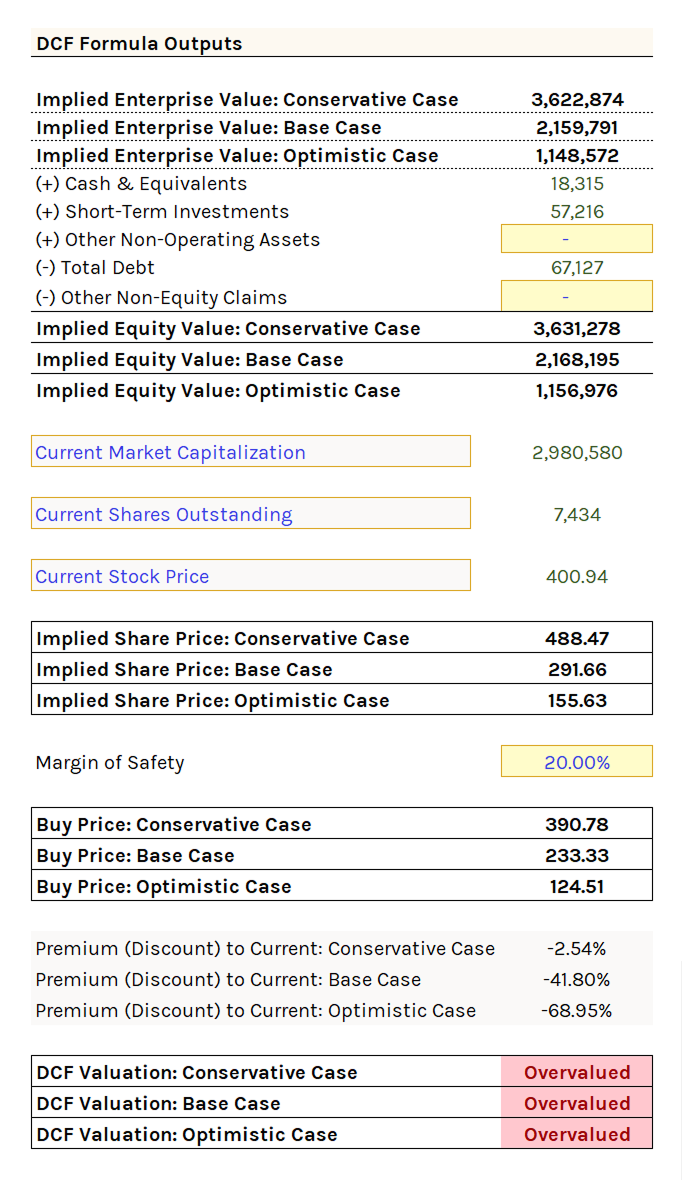
FCFF
Converts implied enterprise value (sum of discounted FCFFs) to implied equity value:
Implied Equity Value = Implied Enterprise Value + Cash & Equivalents + Short-Term Investments + Other Non-Operating Assets - Total Debt - Other Non-Equity Claims
Other Non-Operating Assets and Other Non-Equity Claims are manual input cells.
Divide implied equity value by shares outstanding (basic or diluted) to get the implied share price.
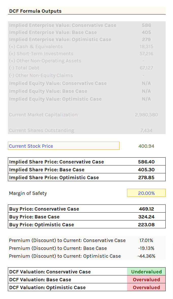
OE
No bridge calculation needed. OE is a levered figure, so cash flows already belong to equity holders.
Implied equity value equals the sum of discounted OE values. Divide by shares outstanding for implied share price.
DEPS
Since DEPS is already per-share, no division by shares outstanding is needed.
Implied share price equals the sum of discounted DEPS values.
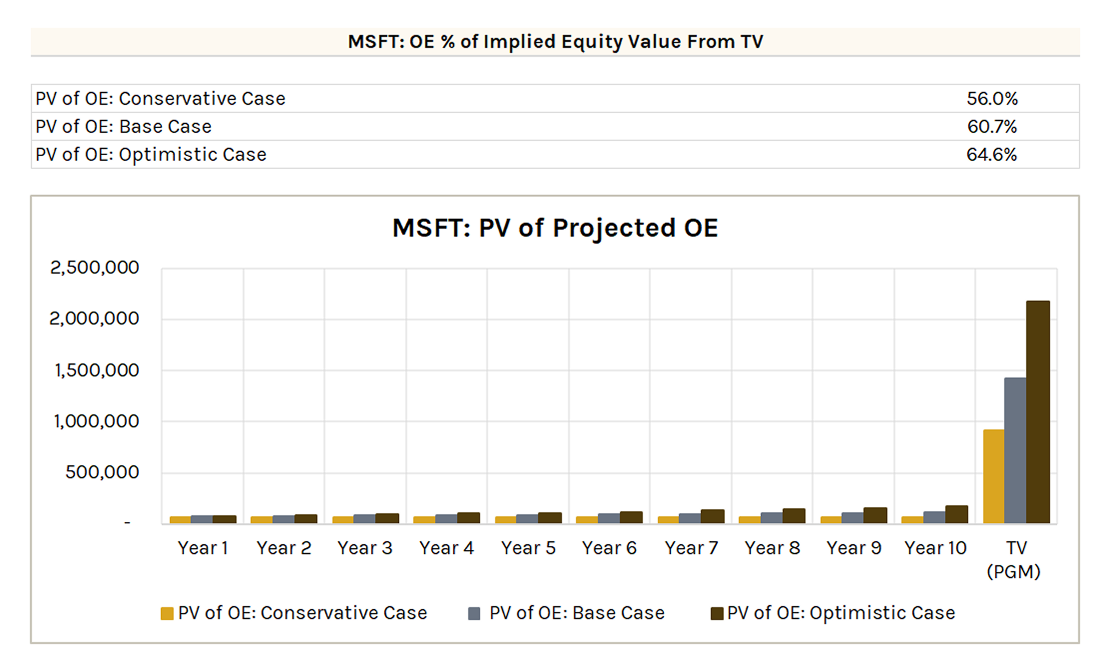
Forecast Method Growth Chart
Shows how the chosen forecast method (FCFF, OE, or DEPS) grows over the forecast period through the terminal value year, after discounting to present value.
Also displays what percentage of total implied value comes from terminal value vs. forecast period cash flows across all three scenarios.
Margin of Safety and Buy Price
Margin of safety (MoS) creates a buffer between intrinsic value and your purchase price to protect against valuation errors:
Buy Price = Implied Share Price × (1 - Margin of Safety %)
The model compares buy price to stock price to determine valuation:
- Undervalued: Buy Price > Stock Price
- Overvalued: Buy Price < Stock Price
The degree of mispricing is calculated as the percentage difference between buy price and stock price across all three scenarios.
Note: If you converted currencies on the OVERVIEW tab, the stock price automatically reflects the FX conversion.
Buy Price vs. Stock Price
Compares the stock price to the calculated buy price. Toggle between conservative, base, and optimistic cases.
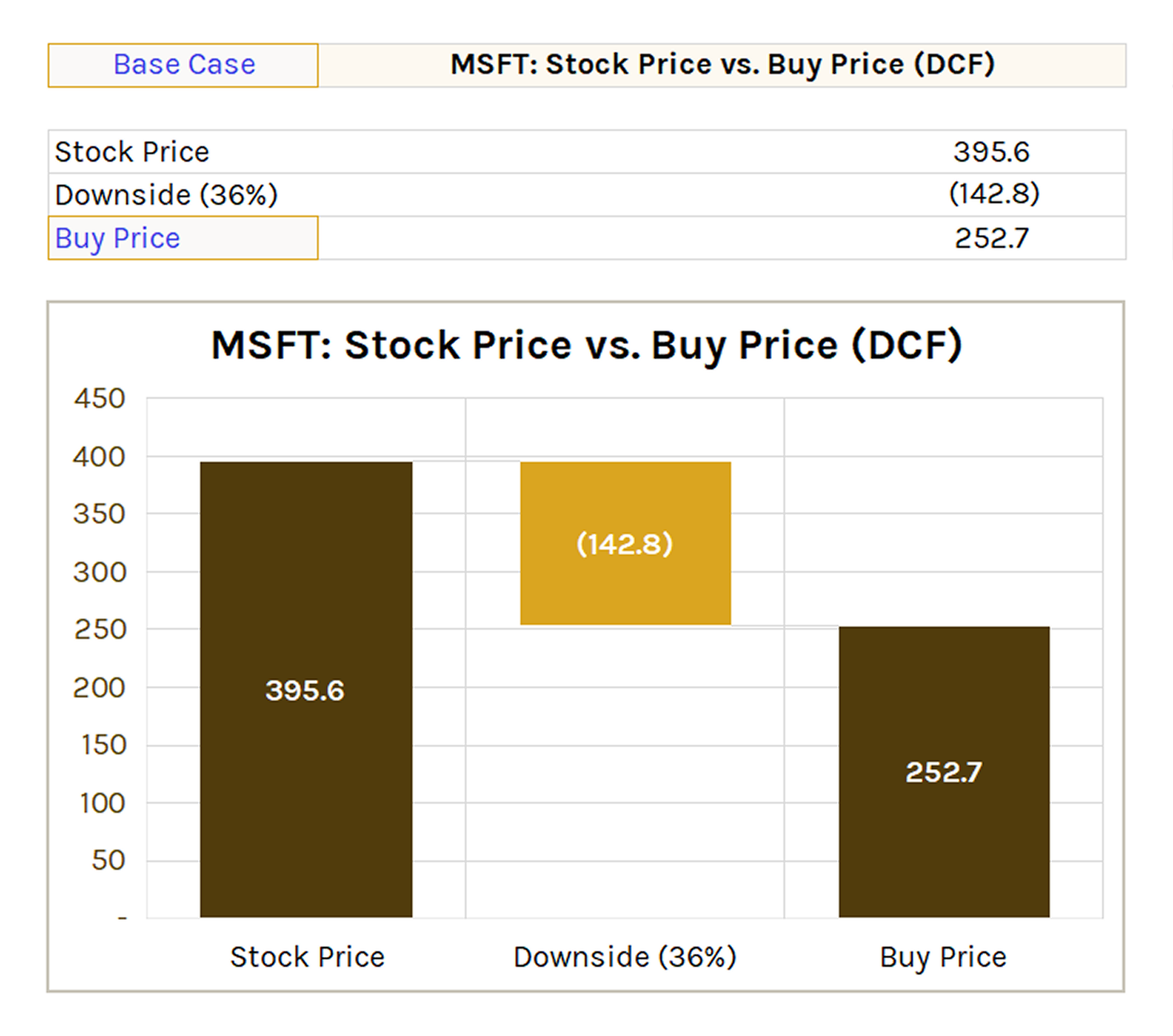
You can also switch from buy price to implied share price to see the valuation before margin of safety.
Sensitivity Analysis
Measures how changes in key DCF inputs affect the buy price, helping establish a valuation range rather than a single point estimate.
Sensitivity Analysis: Discount Rate vs. Perpetual Growth Rate
Two-variable data table showing buy prices across different discount rate and perpetual growth rate combinations. Only applies when using PGM.
Toggle between conservative, base, and optimistic cases. Enter the delta (Δ) increments for each variable.
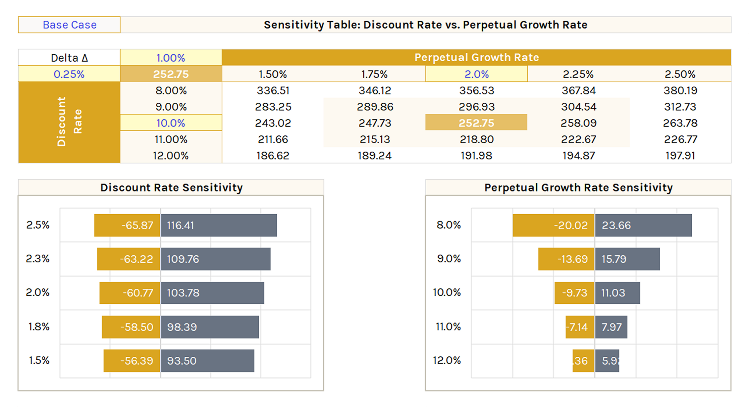
Waterfall charts below isolate the dollar impact of changing each variable independently from the base case. Left bar = decrease in buy price, right bar = increase.
Useful for seeing which input has more impact on valuation and by how much.
Sensitivity Analysis: Discount Rate vs. Margin of Safety
Same format, but compares discount rate changes against margin of safety changes.
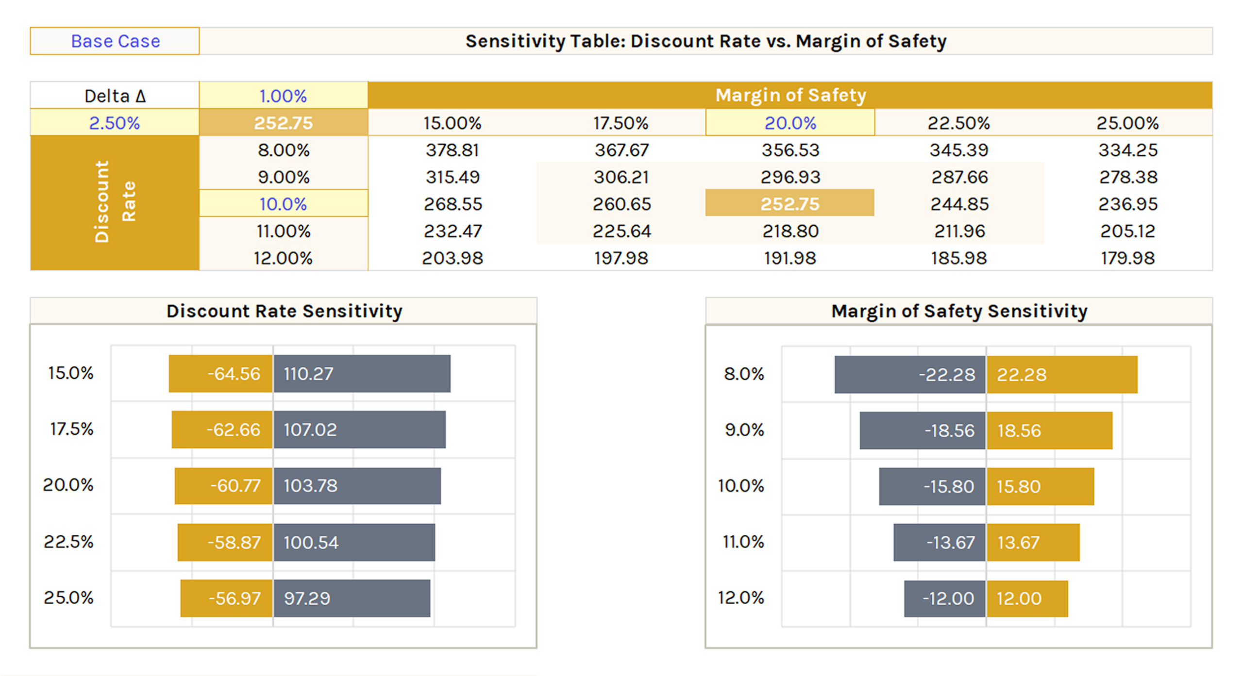
Waterfall charts below follow the same structure.